Use percentiles to analyze application performance

The most common metric used in monitoring or analyzing an application is averages, simply because they are easy to understand and calculate. This topic shows why percentiles are better than averages.

The average response time

This is the most commonly used metric in application performance management. The average response time represents a normal transaction only when the response time is always the same (that is, all transactions run at equal speed) or the response time distribution is roughly bell curved.

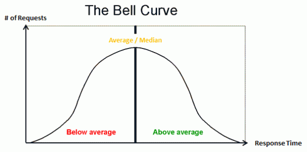
In a bell curve, the average (mean) and median are the same, which means that the observed performance represents only the majority of the transactions.

However, in reality, most applications have fewer heavy outliers, also known as a long tail. A long tail does not imply many slow transactions but only a few that are slower than the norm.

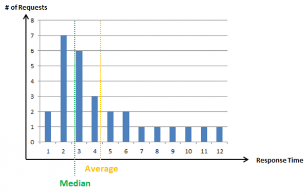
An average does not represent the bulk of transactions but can be a lot higher than the median, which may not be a problem as long as the average doesn't look better than the median. Let's use an real-world scenario to understand this better:

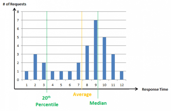
In this case, a considerable percentage of transactions is very fast (10-20 percent) while the bulk of them are several times slower. While the median represents the true story, the average suddenly looks a lot faster than the actual speed of the transactions. This is very typical in search engines when caches are involved; some transactions are super fast but the bulk of them are normal. Another example of this scenario is failed transactions, specifically transactions that failed fast. Most real-world applications have a failure rate of 1-10 percent due to user and validation errors. These failed transactions are often magnitudes faster than the real ones and consequently distort the average.

Performance analysts try to compensate with higher frequency charts by looking at smaller aggregates visually and by considering minimum and maximum observed response times. However, to do this, an in-depth understanding of the product is required. This is why, percentiles are a much better metric.

Automatic baselining and alerting

In real-world environments, performance gets attention only when it is poor and has a negative impact on the business. However, each slow transaction cannot be alerted and manually setting thresholds for multiple applications can be quite cumbersome.

The answer to this is automatic baselining, which calculates the normal performance and sends alerts only when an application slows down or produces more errors than usual. Most approaches rely on averages and standard deviations.

Automatic baselining again, however, assumes that response times are distributed across a bell curve.

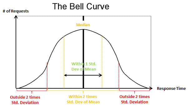
Transactions that are outside 2 times the standard deviation are treated as slow and captured for analysis. An alert is raised only when the average moves significantly. In a bell curve, this accounts for the slowest 16.5 percent, which can be adjusted. However, if the response time distribution does not represent a bell curve it becomes inaccurate. In this case, a lot of false positives (transactions that are much slower than the average but fall within the norm) are alerted or a lot of problems (false negatives) are missed. Also, if the curve is not a bell curve, the average can differ a lot from the median. Applying a standard deviation to such an average can lead to quite a different result than expected.

Percentiles are better

A percentile helps in identifying the exact part of the curve you may be interested in and also the number of transactions that are represented by that metric. To understand this better, look at the following chart:

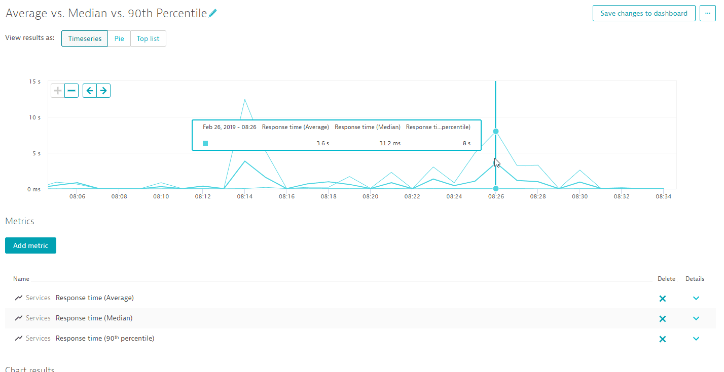
In the above graph, the average seems very volatile. The other two lines represent the median and the response time. The median looks mostly stable with occasional jumps. These jumps indicate degradation in performance for the majority (50%) of the transactions. The response time (90th percentile) is much more volatile, which means that the outliers slowness depends on data or user behavior. The average, however, is heavily influenced by the 90th percentile rather than the bulk of the transactions.

If the median of a response time is 500ms, 50% of transactions are either as fast as or faster than 500ms. If the 90th percentile of the same transaction is at 1000ms, 90% of transactions are fast and the remaining 10% are slow. The average in this case could be lower than 500ms (on a heavy front curve), a lot higher (a long tail), or somewhere in between. A percentile gives a much better sense of the real-world performance because it shows a slice of the response time curve.

Percentiles, therefore, are perfect for automatic baselining. If the median moves from 500ms to 600ms, 50% of transactions can be assumed to have suffered a 20% performance degradation.

In most cases, the 70th or the 90th percentile does not change at all. This means that the slow transactions didn't get any slower, only the normal ones did. Depending on how long the tail is, the average might have not moved at all in these cases.

In other cases, the 98th percentile degrades from 1 to 1.5 seconds while the 95th percentile is stable at 900ms. This means that the application as a whole is stable, but a few outliers are getting worse.

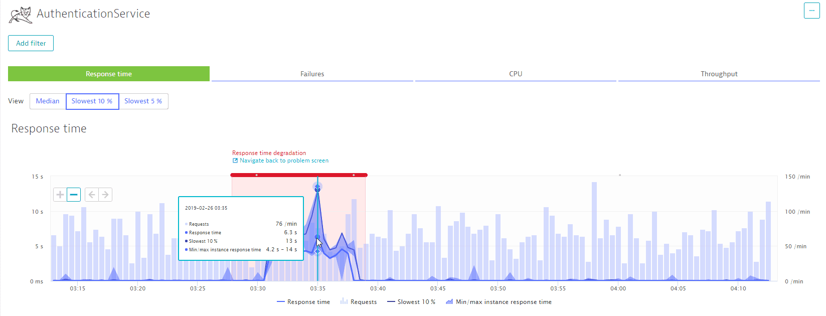
The following screen explains how percentile-based alerts do not suffer from false positives, are a lot less volatile, and don't miss important performance degradation.

Percentiles for tuning

Percentiles set goals for optimizations. If something in the application is slow and needs to be set up, the 90th percentile should be brought down. This would ensure that the overall response time of the application goes down. In the case of unacceptably long outliers, the response time for transactions beyond the 98th or the 99th percentile should be brought down. A lot of applications that have perfectly acceptable performance for the 90th percentile with the 98th percentile being worse by magnitudes.

In throughput-oriented applications, however, the focus should be on making the majority of transactions very fast, while accepting that an optimization makes a few outliers slower. Therefore, it should be ensured that the 75th percentile goes down and the 90th percentile remains stable or at least does not get a lot worse.

While the same kind of observation could be derived from averages, minimum, and maximum, doing so with percentiles is much easier.