Analyzing Java Memory

The goal of any Java memory analysis is to optimize garbage collection (GC) in such a way that its impact on application response time or CPU usage is minimized. It is equally important to ensure the stability of the application. Memory shortages and leaks often lead to instability. To identify memory-caused instability or excessive garbage collection we first need to monitor our Java application with appropriate tools. If garbage collection has a negative impact on response time, our goal must be to optimize the configuration. The goal of every configuration change must be to decrease that impact. Finally, if configuration changes alone are not enough we must analyze the allocation patterns and memory usage itself. So let's get to it.

Since Java 5, the standard JDK monitoring tool has been JConsole. The Oracle JDK also includes jStat, which enables the monitoring of memory usage and garbage-collector activity from the console, and Java VisualVM (or jvisualvm), which provides rudimentary memory analyzes and a profiler. The Oracle JRockit JDK includes JRockit Mission Control and the verbose:gc flag of the JVM. Each JVM vendor includes its own monitoring tools, and there are numerous commercial tools available that offer additional functionality.

Memory shortage is often the cause of instability and unresponsiveness in a Java applications. Consequently, we need to monitor the impact of garbage collection on response time and memory usage to ensure both stability and performance. However, monitoring memory utilization and garbage collection times is not enough, as these two elements alone do not tell us if the application response time is affected by garbage collection. Only GC suspensions affect response time directly, and a GC can also run concurrent to the application. We therefore need to correlate the suspensions caused by garbage collection with the application's response time. Based on this we need to monitor the following:

• Utilization of the different memory pools (Eden, survivor, and old). Memory shortage is the number-one reason for increased GC activity.
• If overall memory utilization is increasing continuously despite garbage collection, there is a memory leak, which will inevitably lead to an out-of-memory error. In this case, a memory heap analysis is necessary.
• The number of young-generation collections provides information on the churn rate (the rate of object allocations). The higher the number, the more objects are allocated. A high number of young collections can be the cause of a response-time problem and of a growing old generation (because the young generation cannot cope with the quantity of objects anymore).
• If the utilization of the old generation fluctuates greatly without rising after GC, then objects are being copied unnecessarily from the young generation to the old generation. There are three possible reasons for this: the young generation is too small, there's a high churn rate, or there's too much transactional memory usage.
• High GC activity generally has a negative effect on CPU usage. However, only suspensions (aka stop-the-world events) have a direct impact on response time. Contrary to popular opinion, suspensions are not limited to major GCs. It is therefore important to monitor suspensions in correlation to the application response time.

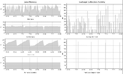
The JVM memory dashboard (Figure 2.11) shows that the tenured (or old) generation is growing continuously, only to drop back to its old level after an old-generation GC (lower right). This means that there is no memory leak and the cause of the growth is prematurely-tenured objects. The young generation is too small to cope with the allocations of the running transactions. This is also indicated by the high number of young-generation GCs (Oracle/Sun Copy GC). These so-called minor GCs are often ignored and thought to have no impact.

The JVM will be suspended for the duration of the minor garbage collection; it's a stop-the-world event. Minor GCs are usually quite fast, which is why they are called minor, but in this case they have a high impact on response time. The root cause is the same as already mentioned: the young generation is too small to cope. It is important to note that it might not be enough to increase the young generation's size. A bigger young generation can accommodate more live objects, which in turn will lead to longer GC cycles. The best optimization is always to reduce the number of allocations and the overall memory requirement.

Of course, we cannot avoid GC cycles, and we would not want to. However, we can optimize the configuration to minimize the impact of GC suspensions on response time.

GC suspensions represent the only direct impact on response time by the garbage collector. The only way to monitor this is via the JVM tool interface (JVM TI), which can be used to register callbacks at the start and end of a suspension. During a stop-the-world event, all active transactions are suspended. We can correlate these suspensions to application transactions by identifying both the start and end of the suspension. Effectively, we can tell how long a particular transaction has been suspended by the GC. (See Figure 2.12.)

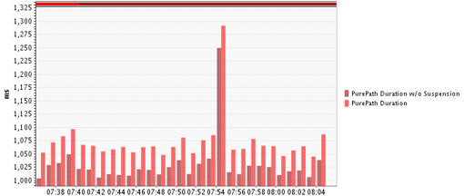
Only a handful of tools allow the direct monitoring of suspensions, Dynatrace being one of them. If you do not have such a tool you can use jStat, JConsole, or a similar tool to monitor GC times. The metrics reported in jStat are also directly exposed by the JVM via JMX. This means you can use any JMX-capable monitoring solution to monitor these metrics.

It is important to differentiate between young- and old-generation GCs (or minor and major, as they are sometimes called; see more in the next section) and equally important to understand both the frequency and the duration of GC cycles. Young-generation GCs will be mostly short in duration but under heavy load can be very frequent. A lot of quick GCs can be as bad for performance as a single long-lasting one (remember that young-generation GCs are always stop-the-world events).

Frequent young-generation GCs have two root causes:

• A too-small young generation for the application load.
• High churn rate

If the young generation is too small, we see a growing old generation due to prematurely tenured objects.

If too many objects are allocated too quickly (i.e., if there's a high churn rate), the young generation fills up as quickly and a GC must be triggered. While the GC can still cope without overflowing to the old generation, it has to do so at the expense of the application's performance.

A high churn rate might prevent us from ever achieving an optimal generation sizing, so we must fix such a problem in our code before attempting to optimize garbage collection itself. There is a relatively easy way to identify problematic code areas.

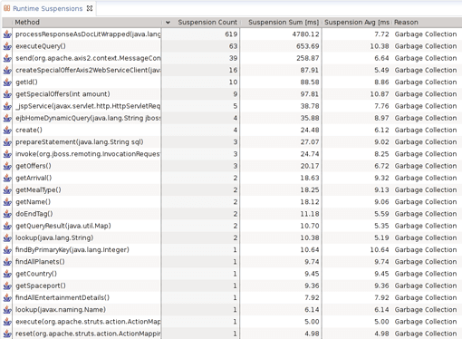
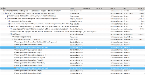
The runtime suspensions shown in Figure 2.13 report a massive statistical concentration of garbage collections in one particular function. This is very unusual, because a GC is not triggered by a particular method, but rather by the fillstate of the heap. The fact that one method is suspended more than others suggests that the method itself allocates enough objects to fill up the young generation and thus triggers a GC. Whenever we see such a statistical anomaly we find a prime candidate for allocation analysis and optimization (which we'll examine further in the Allocation Analysis section of this chapter, below).

What I have been referring to as young- and old-generation GCs, are commonly referred to as minor and major GCs. Similarly, it is common knowledge that major GCs suspend your JVM, are bad for performance, and should be avoided if possible. On the other hand, minor GCs are often thought to be of no consequence and are ignored during monitoring. As already explained, minor GCs suspend the application and neither they nor major GCs should be ignored. A major GC is often equated with garbage collection in the old generation; this is, however, not fully correct. While every major GC collects the old generation, not every old-generation GC is a major collection. Consequently, the reason we should minimize or avoid major GCs is misunderstood. Looking at the output of verbose:GC explains what I mean:

 [GC 325407K->83000K(776768K), 0.2300771 secs]
 [GC 325816K->83372K(776768K), 0.2454258 secs]
 [Full GC 267628K->83769K(776768K), 1.8479984 secs]

A major GC is a full GC. A major GC collects all areas of the heap, including the young generation and, in the case of the Oracle HotSpot JVM, the permanent generation. Furthermore, it does this during a stop-the-world event, meaning the application is suspended for a lengthy amount of time, often several seconds or minutes. On the other hand, we can have a lot of GC activity in the old generation without ever seeing a major (full) GC or having any lengthy GC-caused suspensions. To observe this, simply execute any application with a concurrent GC. Use jstat—gcutil to monitor the GC behavior of your application.

This output is reported by jstat -gcutil. The first five columns in Table 2.1 show the utilization of the different spaces as a percentage—survivor 0, survivor 1, Eden, old, and permanent—followed by the number of GC activations and their accumulated times—young GC activations and time, full GC activations and time. The last column shows the accumulated time used for garbage collection overall. The third row shows that the old generation has shrunk and jStat reported a full GC (see the bold numbers).

**S0** **S1** **E** **O** **P** **YGC** **YGCT** **FGC** **FGCT** **GCT**
90.68 0.00 32.44 85.41 45.03 134 15.270 143 21.683 36.954
90.68 0.00 32.45 85.41 45.03 134 15.270 143 21.683 36.954
90.68 0.00 38.23 _**85.41**_ 45.12 134 15.270 _**143**_ _**21.683**_ _**36.954**_
90.68 0.00 38.52 _**85.39**_ 45.12 134 15.270 _**144**_ _**21.860**_ _**37.131**_
90.68 0.00 38.77 85.39 45.12 134 15.270 144 21.860 37.131
90.68 0.00 49.78 85.39 45.13 134 15.270 145 21.860 37.131

Table 2.1: jstat -gcutil output report

On the other hand, monitoring the application with JConsole (Figure 2.14), we see no GC runs reported for the old generation, although we see a slightly fluctuating old generation.

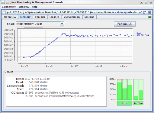
Which of the two tools, jStat (Figure 2.13) or JConsole (Figure 2.14) is correct?

In fact, both are only partially correct, which is rather misleading. as reported by jStat, the concurrent GC has executed, but it has done so asynchronously to the application and for the old generation only, which is its purpose. It was not a full GC! JStat reports old-generation GCs as full GCs, which is wrong. This is most likely a legacy from days prior to concurrent and incremental GCs.

JConsole reports activations via Java Management Extensions (JMX) and managed beans (MBeans). Previously, these MBeans reported only real major GCs. In the case of the CMS, these occur only when the CMS is not able to do its work concurrent to the application, due to memory fragmentation or high churn rate. For this reason, JConsole would not show any activations.

In a recent release the CMS, Memory MBean has been changed to report only activations of the CMS itself; the downside is that we have no way to monitor real major GCs anymore.

In the IBM WebSphere JVM, major and minor GCs are indistinguishable via JConsole. The only way to distinguish between them is by using the verbose:gc flag.

For these reasons, we mistakenly ignore minor GCs and overrate old-generation GCs by considering them to be major. The truth is we need to monitor JVM suspensions and understand whether the root causes lie in the young generation, due to object churn, or the old generation, due to wrong sizing or a memory leak.

We have discussed the impact of suspensions have on application response time. However, transaction rates or more important for throughput or batch applications. Consequently we do not care about the pause-time impact to a particular transaction, but about the CPU usage and overall suspension duration.

Consider the following. In a response-time application it is not desirable to have a single transaction suspended for 2 seconds. It is, however, acceptable if each transaction is paused for 50 ms. If this application runs for several hours the overall suspension time will, of course, be much more than 2 seconds and use a lot of CPU, but no single transaction will feel this impact! The fact that a throughput application cares only about the overall suspension and CPU usage must be reflected when optimizing the garbage-collection configuration.

To maximize throughput the GC needs to be as efficient as possible, which means executing the GC as quickly as possible. As the whole application is suspended during the GC, we can and should leverage all existing CPUs. At the same time we should minimize the overall resource usage over a longer period of time. The best strategy here is a parallel full GC (in contrast to the incremental design of the CMS).

It is difficult to measure the exact CPU usage of the garbage collection, but there's an intuitive shortcut. We simply examine the overall GC execution time. This can be easily monitored with every available free or commercial tool. The simplest way is to use jstat -gc 1s. This will show us the utilization and overall GC execution on a second-by-second basis (see Table 2.2).

**S0** **S1** **E** **O** **P** **YGC** **YGCT** **FGC** **FGCT** **GCT**
0.00 21.76 69.60 9.17 75.80 **63** **2.646** **20** **9.303** **11.949**
0.00 21.76 71.24 9.17 75.80 **63** **2.646** **20** **9.303** **11.949**
0.00 21.76 71.25 9.17 75.80 **63** **2.646** **20** **9.303** **11.949**
0.00 21.76 71.26 9.17 75.80 **63** **2.646** **20** **9.303** **11.949**
0.00 21.76 72.90 9.17 75.80 **63** **2.646** **20** **9.303** **11.949**
0.00 21.76 72.92 9.17 75.80 **63** **2.646** **20** **9.303** **11.949**
68.74 0.00 1.00 9.17 76.29 _**64**_ **2.719** **20** **9.303** _**12.022**_
68.74 0.00 29.97 9.17 76.42 **64** **2.719** **20** **9.303** **12.022**
68.74 0.00 31.94 9.17 76.43 **64** **2.719** **20** **9.303** **12.022**
68.74 0.00 33.42 9.17 76.43 **64** **2.719** **20** **9.303** **12.022**

Table 2.2: Rather than optimizing for response time, we need only look at the overall GC time.

Using graphical tools, the GC times can be viewed in charts and thus correlated more easily with other metrics, such as throughput. In Figure 2.15 we see that while the garbage collector is executed, suspending quite often in all three applications, it consumes the most time in the GoSpaceBackendit this does not seem to have an impact on throughput.

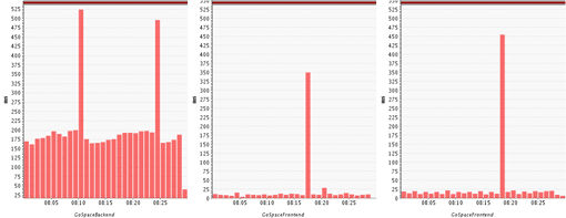
It can be safely assumed that it also requires far more CPU resources than in the other JVMs and has a higher negative impact. With increasing load, the GC times will also rise; this is normal! However, the GC time should never take up more than 10% of the total CPU time used by the application. If CPU usage rises disproportionately to application load, or if the usage is disproportionately heavy, one must consider a change in the GC configuration or an improvement in the application.

Allocating objects in Java is relatively inexpensive compared to C++, for instance. The generational heap is specifically geared for fast and frequent allocations of temporary objects. But it's not free! Allocations can quickly become a choke point when a lot of concurrent threads are involved. Reasons include memory fragmentation, more frequent GCs due to too many allocations, and synchronization due to concurrent allocations. Although you should refrain from implementing object pools for the sole sake of avoiding allocations, not allocating an object is the best optimization.

The key is to optimize your algorithms and avoid making unnecessary allocations or allocating the same object multiple times. For instance, we often create temporary objects in loops. Often it is better to create such an object once prior to the loop and just use it. This might sound trivial, but depending on the size of object and the number of loop recursions, it can have a high impact. And while it might be the obvious thing to do, a lot of existing code does not do this. It is a good rule to allocate such temporary "constants" prior to looping, even if performance is no consideration.

Allocation analysis is a technique of isolating areas of the application that create the most objects and thus provide the highest potential for optimization. There are a number of free tools, such as JVisualVM], for performing this form of analysis. You should be aware that these tools all have enormous impact on runtime performance and cannot be used under production-type loads. Therefore we need to do this during QA or specific performance-optimization exercises.

It is also important to analyze the correct use cases, meaning it is not enough to analyze just a unit test for the specific code. Most algorithms are data-driven, and so having production-like input data is very important for any kind of performance analysis, but especially for allocation analysis.

Let's look at a specific example. I used JMeter to execute some load tests against one of my applications. Curiously, JMeter could not generate enough load and I quickly found that it suffered from a high level of GC activity. The findings pointed towards a high churn rate (lots of young-generation GCs). Consequently I used an appropriate tool (in my case, JVisualVM) to do some allocation hot-spot analysis. Before I go into the results, I want to note that it is important to start the allocation analysis after the warm-up phase of a problem. A profiler usually shows hotspots irrespective of time or transaction type. We do not want to skew those hot spots with data from the initial warm-up phase (caching and startup). I simply waited a minute after the start of JMeter before activating the allocation analysis. The actual execution timing of the analysis application must be ignored; in most cases the profiler will lead to a dramatic slowdown.

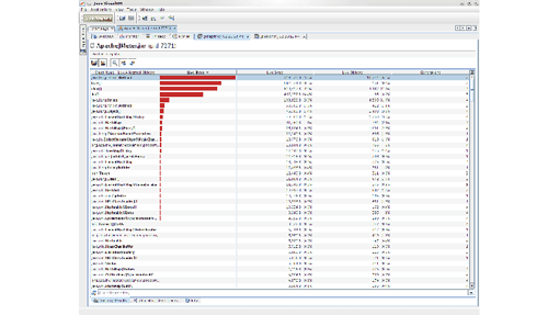
The analysis (Figure 2.16) shows which types of objects are allocated most and where these allocations occur. Of primary interest are the areas that create many or large objects (large objects create a lot of other objects in their constructor or have a lot of fields). We should also specifically analyze code areas that are known to be massively concurrent under production conditions. Under load, these locations will not only allocate more, but they will also increase synchronization within the memory management itself. In my scenario I found a huge number of Method objects were allocated (Figure 2.16). This is especially suspicious because a Method object is immutable and can be reused easily. There is simply no justification to have so many new Method objects.

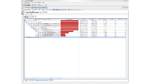
By looking at the origin of the allocation (Figure 2.17), I found that the Interpreter object was created every time the script was executed instead of being reused. This led to the allocations of the Method objects. A simple reuse of that Interpreter object removed more than 90% of those allocations.

To avoid going quickly astray, it is important to check each optimization for a positive effect. The transaction must be tested before and after the optimization under full load and, naturally, without the profiler, and the results compared against each other. This is the only way to verify the optimization.

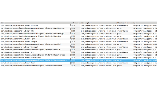
Some commercial tools, such as Dynatrace (see Figures 2.18 and 2.19), also offer the ability to test allocations on a transaction basis under load conditions. This has the added advantage of taking into account data-driven problems and concurrency issues, which are otherwise difficult to reproduce in a development setup.

So far we have dealt with the influence of garbage collection and allocations on application performance. I have stated repeatedly that high memory utilization is a cause for excessive garbage collection. In many cases, hardware restrictions make it impossible to simply increase the heap size of the JVM. In other cases increasing the heap size does not solve but only delays the problem because the utilization just keeps growing. If this is the case, it is time to analyze the memory usage more closely by looking at a heap dump.

A heap dump is a snapshot of main memory. It can be created via JVM functions or by using special tools that utilize the JVM TI. Unfortunately, JVM-integrated heap dumps are not standardized. Within the Oracle HotSpot JVM, one can create and analyze heap dumps using jmap, jhat, and VisualVM. JRockit includes its JRockit Mission Control, which offers a number of functions besides memory analysis itself.

The heap dump itself contains a wealth of information, but it's precisely this wealth that makes analysis hard—you get drowned easily in the quantity of data. Two things are important when analyzing heap dumps: a good Tool and the right technique. In general, the following analyzes are possible:

• Identification of memory leaks
• Identification of memory eater

Every object that is no longer needed but remains referenced by the application can be considered a memory leak. Practically we care only about memory leaks that are growing or that occupy a lot of memory. A typical memory leak is one in which a specific object type is created repeatedly but not garbage-collected (e.g., because it is kept in a growing list or as part of an object tree). To identify this object type, multiple heap dumps are needed, which can be compared using trending dumps.

Trending dumps only dump a statistic of the number of instances on the class level and can therefore be provided very quickly by the JVM. A comparison shows which object types have a strongly rising tendency. Every Java application has a large number amount of String, char[], and other Java-standard objects. In fact, char[] and String will typically have the highest number of instances, but analyzing them would take you nowhere. Even if we were leaking String objects, it would most likely be because they are referenced by an application object, which represents the root cause of the leak. Therefore concentrating on classes of our own application will yield faster results.

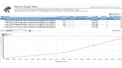
Figure 2.20 shows a view on multiple trending dumps that I took from a sample application I suspected of having a memory leak. I ignored all standard Java objects and filtered by my application package. I immediately found an object type that constantly increased in number of instances. As the object in question was also known to my developer, we knew immediately that we had our memory leak.

There are several cases when you want to do a detailed memory analysis.

• The Trending Analysis did not lead you to your memory leak
• Your application uses to much memory, but has no obvious memory leak, and you need to optimize
• You could not do a trending analysis because memory is growing too fast and your JVM is crashing

In all three cases the root cause is most likely one or more objects that are at the root of a larger object tree. These objects prevent a whole lot of other objects in the tree from being garbage-collected. In case of an out-of-memory error it is likely that a handful of objects prevent a large number of objects from being freed, hence triggering the out-of-memory error. The purpose of a heap-dump analysis is to find that handful of root objects.

The size of the heap is often a big problem for a memory analysis. Generating a heap dump requires memory itself. If the heap size is at the limit of what is available or possible (32-bit JVMs cannot allocate more than 3.5 GB), the JVM might not be able to generate one. In addition, a heap dump will suspend the JVM. Depending on the size, this can take several minutes or more. It should not be done under load.

Once we have the heap dump we need to analyze it. It is relatively easy to find a big collection. However, manually finding the one object that prevents a whole object tree (or network) from being garbage-collected quickly becomes the proverbial needle in a haystack.

Fortunately solutions like Dynatrace are able to identify these objects automatically. To do this they use a dominator algorithm that stems from graph theory. This algorithm is able to calculate the root of an object tree. In addition to calculating object-tree roots, the memory-analysis tool calculates how much memory a particular tree holds. This way it can calculate which objects prevent a large amount of memory from being freed—in other words, which object dominates memory (see Figure 2.21).

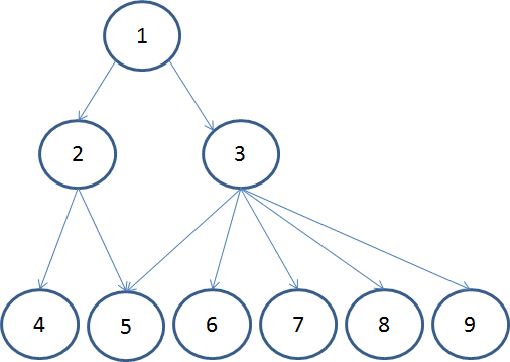
Let us examine this using the example in Figure 2.21. Object 1 is the root of the displayed object tree. If object 1 no longer references object 3, all objects that would be kept alive by 3 are garbage-collected. In this sense, object 3 dominates objects 6 ,7 ,8, and 9. Objects 4 and 5 cannot be garbage-collected because they are still referenced by one other (object 2). However, if object 1 is dereferenced, all the objects shown here will be garbage-collected. Therefore, object 1 dominates them all.

A good tool can calculate the dynamic size of object 1 by totaling the sizes of all the objects it dominates. Once this has been done, it is easy to show which objects dominate the memory. In Figure 2.21, objects 1 and 3 will be the largest hot spots. A practical way of using this is in a memory hotspot view as we have in Figure 2.22:

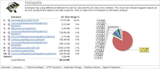
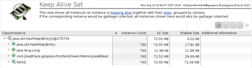
The HashMap$Entry array dominates—it accounts for more than 80 percent of the heap. Were it to be garbage-collected, 80% of our heap would be empty. From here it is a relative simple matter to use the heap dump to figure out why. We can then easily understand and show why that object itself has not been garbage-collected. Even more useful is to know which objects are being dominated and make up that hot spot. In Dynatrace we call this the Keep Alive Set (see Figure 2.23).

With the aid of such analyzes, it is possible to determine within a few minutes whether there is a large memory leak or whether the cache uses too much memory.