Calculating Performance Data

Performance analysis is always based on numbers. In many cases we are not working with "raw values" but rather aggregated data. If each measurement were viewed indi-vidually, you couldn't see the forest for the trees. At the same time certain measure-ment approaches, like JMX (which we will discuss later), only provide us with aggregated data.

Understanding how a value is calculated and what this means is essential for drawing the right conclusions. Toward this end, we must examine the statistical methods used to calculate and aggregate performance data.

The average is the most basic and also most widely used data representation and is built into every performance tool. It is likely the most overused measure, because it can only provide a "first impression" of performance. For instance, the average of a series of volatile measurements, where some values are very low and others very high, can easily be skewed by outliers. So while the average might look good, it can fail to reveal an actual performance problem.

The aggregation interval can skew things even further. When measurement data is subject to time fluctuations over longer durations, the average can't reflect this information and loses it's mean-ing. Similarly, over a very short period in which only a small number of measurements is taken, average is simply statistically imprecise.

For example, if we examine the response time of an application over a period of 24 hours, the peak values will be hidden by the average. Measurements taken when the system was under low load having good response times will "average out" times of peak system load.

Minimum and maximum values give us a measure of both extremes and the spread of these extremes. Since there are always outliers in any measurement, they are not necessarily very meaningful. In practice this data is rarely used, as it does not provide a basis for determining how often the corresponding value has actually occurred. It might have occurred one time or a hundred times.

The main use of these values is to verify how high the quality of the calculated average value is. If these values are very close, it can be assumed that the average is representative for the data.

In applications with demanding performance requirements, the maximum is still often used instead of, or in addition to, the average to check whether the response times lie below a certain level. This is especially true for applications which must never exceed certain thresholds.

The median or middle value of a series of numbers is another widely used representation of performance data. It is also called the 50th percentile; In a series of 89 measurements, the median would be the 45th measurement. The advantage of the median is that it is closer to real world data and not an artificially calculated value like the average which is strongly influenced by outliers. The impact of outliers on the median is much lower than on the average.

Taken by itself, average has only limited significance. However, it's considerably more meaningful when use with standard deviation. The standard deviation measures the spread of actual values. The greater the standard deviation, the larger is the difference in the measurement data. Assuming that our values are distributed normally, at least two thirds of all values will fall within the range covered by the average plus/minus one standard deviation.

When working with the standard deviation, we assuming the data is normally distributed. If our data does not follow this distribution, then the standard deviation is meaningless. This means that we have to understand the characteristics of the underlying data before we rely on statistically derived metrics.

The figure below shows an example of the response time distribution of an application. We can clearly see that these values are not normally distributed. In this case, using average with standard deviation will give us incorrect wrong conclusions.

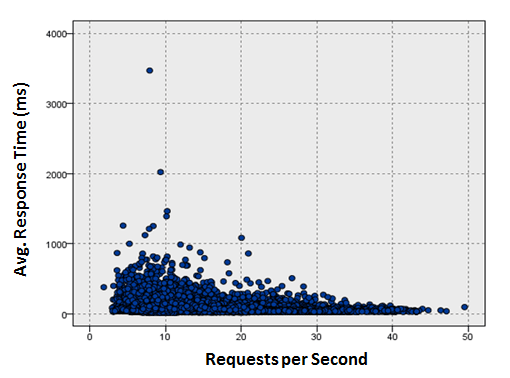
There are many causes for this kind of variation in measurement data. For instance, genuinely volatile response times probably in-dicate a problem with the application. Another possibility is that the individual requests differ in what they are actually doing. We might have also combined data points into single measurements which measure different things.

For example, when examining the response times of a portal start page, our data will vary greatly depending on how many portlets are open in each instance. For some users, there may be only one or two, while for others, there can be twenty or more per page. In this case, it is not possible to draw reasonable conclusions about the response times of the start page, because there is no specific "start page." The only way to get meaningful measurements in this case is to aggregate the measurements differently. For instance, we could group measurement data by the number of portlets that are shown on a page.

Percentiles are probably the most precise, but also the most difficult to calculate representation of data. Percentiles define the maximum value for a percentage of the overall measurements. If the 95th percentile for the application response time is two seconds, this means that 95% of all response times were less than or equal to two seconds.

Higher percentile values, meaning the 95th to 98th, are often used instead of the average. This can eliminate the impact of outliers and provide a good representation of the underlying raw data.

The concept for the calculation is very simple and similar to the median. The difference is that we not only divide the measurements at 50 percent, but according to the percentile ranges. So the 25th percentile means that we take the lowest 25 percent of all measured values.

The difficulty lies in calculating percentiles in real time for a large number of values: more data is necessary for this calculation com-pared to the average, which requires only the sum and the number of values. If it is possible to work with percentiles, they should definitely be used. Their meaning is easier to understand than the average combined with standard deviation resulting in faster and better analysis