
Visualizing Performance Data
Chapter: Application Performance Concepts

In addition to measuring performance data, we also have to visualize it for analysis. Depending on the underlying data structure, we differentiate two types of data for visualization:
- Time-based data, like JMX values, are represented as relations, or tuples, where the data value is paired with a timestamp. So for each measurement of, for example, CPU load, network usage, or transaction count, there can only be a single value or data point. Depending on the use case, we can visualize these data using various chart types: line, meter, traffic lights, whatever it takes to plot this information for a given use case.
- Execution-time data is represented hierarchically as an ordering of methods and associated execution times—a call tree. In fact, all of the execution-time measurements we've mentioned can be visualized as trees. Note however, that the semantics for reading these different trees is not always the same.
We will not cover the representation of time-based monitoring data in further detail as it is quite easy to understand. However, the different representations for execution-time data require a bit more of explanation.
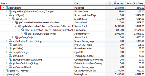
Aggregating Execution Data in Call Trees
Both time-based and event-based execution data can be represented as call trees. This nicely illustrates the call hierarchy, but at the cost of obscuring the actual sequence of individual calls.
Call trees are primarily used to help identify execution hot spots—those areas where methods are called most frequently and have the greatest execution times.
Practically speaking, problems due to high CPU utilization or long wait times caused by lengthy synchronization are easily diagnosed with call trees. However, the loss of call sequence information makes it impossible to use call trees to find logical control flow issues.
On the one hand, using call trees, we should be able to identify an application hot spot caused by a long-running and complex database call. On the other hand, call trees are not likely to illuminate a problem stemming from a high number of cache misses requiring repeated queries of the database. The cache miss method is likely lost in the hotspots, since it does not consume much execution time.
Depending on the performance tool used, you may also have additional information available, such as called database statements, specific URLs, or other important diagnostic data. There is also a certain amount of data and report customization available. Using these data can help to distinguish call data and to enable better and simpler analysis.
With regard to complex performance problems, however, one quickly reaches the limits of this approach.
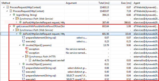
Visualizing Individual Call Traces
Using transactional measurement methods makes it possible to show the call sequence of each transaction or request individually. The visual representation will look very similar to a call tree, but the data is far more precise and therefore the visualization will be more accurate.
Call traces show the timely sequence of method execution, which provides a visual representation of transaction-based logical flow. With this visualization technique, complex problems, like the one described above, are no longer un-diagnosable! Furthermore, as we can see in the example below, this information can also be used to diagnose functional problems, like an exception being thrown in the context of a remote service invocation.
Showing Complex Transactions as Transaction Flows
Particularly in distributed environments, call trace visualizations provide invaluable insight into the dynamic characteristics of application performance. However, when used in a production environment where there's a constant load of thousands of transactions per second, it is no longer feasible to examine individual transactions.
This brings us into the realm of transaction flow visualizations, which, as the name implies, are able to represent the flow of individual or aggregated transactions through an application. As shown in the figure below, this visualization is used to analyze performance problems in complex, high-volume, distributed environments.
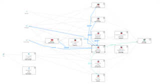
Table of Contents
Application Performance Concepts
Memory Management
How Java Garbage Collection Works
The Impact of Garbage Collection on application performance
Reducing Garbage Collection Pause time
Making Garbage Collection faster
Not all JVMS are created equal
Analyzing the Performance impact of Memory Utilization and Garbage Collection
The different kinds of Java memory leaks and how to analyze them
High Memory utilization and their root causes
Classloader-releated Memory Issues
Performance Engineering
Virtualization and Cloud Performance
Try it free
