Maximize user experience with out-of-the-box service-performance SLOs

The benefits of flexibility, autonomy, and velocity that are provided by microservice-based architectures typically come at the cost of increased complexity of the overall system. Continuously observing service performance is a crucial aspect of ensuring business success. For efficient monitoring of performance levels, service-level objectives (SLOs) provide an essential means of setting and measuring service-quality targets—tracking lagging and leading indicators.

SLOs cover a wide range of monitoring options for different applications. This article explores SLOs for service performance. If you’re new to SLOs and want to learn more about them, how they’re used, and best practices, see the additional resources listed at the end of this article.

According to the Google Site Reliability Engineering (SRE) handbook, monitoring the four golden signals is crucial in delivering high-performing software solutions. These signals (latency, traffic, errors, and saturation) provide a solid means of proactively monitoring operative systems via SLOs and tracking business success.

How to measure performance

SLOs are based on service-level indicators (SLIs), which are used to track performance against pre-defined service-level agreements (SLAs).

While this connection might sound simple, finding the right metrics to measure the needed SLIs takes time and effort. Moreover, after selecting an SLI, complex metric expressions might be required to extract and interpret the result and come to the right conclusions and decisions.

SLOs, as a measure of service quality, can track the related availability, reliability, and performance. Hence, service performance is one key indicator for defining and monitoring service-side objectives. Performance typically addresses response times or latency aspects and contributes to the four golden signals.

Generally, response times measure the total duration of receiving, processing, and completing a request. Among other measures, response times significantly contribute to evaluating frictionless and satisfying user experiences and hence are included in calculating the Application Performance Index (Apdex). Proactively monitoring these indicators is vital to achieving the expected and desired performance.

Service-performance template

Latency is often described as the time a request takes to be served. This is what Dynatrace captures as response time. An excellent way to establish an SLO based on latency is to have a certain percentage of all service requests returned within a selected time frame of, for example, 300 ms. Once the SLI metric is defined, an SLO can be created based on the ratio of high-performing partitions (time intervals) compared to all partitions.

To simplify the process, Dynatrace provides dedicated templates for SLO creation via the SLO Wizard. One template explicitly targets service performance monitoring.

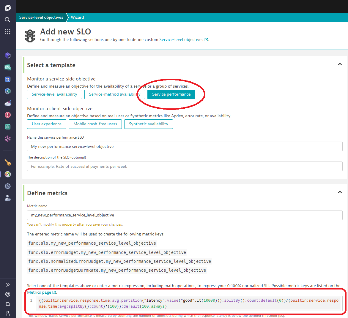
The service performance SLO depicts the ratio of the count of partitions (time intervals) rated as “fast” compared to the total count of all partitions. The respective metric expression looks like this:

((builtin:service.response.time:avg:partition("latency",value("good",lt(10000))):splitBy():count:default(0))/(builtin:service.response.time:avg:splitBy():count)*(100)):default(100,always)

How to use and interpret the template

Looking back to the provided metric expression, different metric transformations, such as avg, partition, splitBy, lt, count, and default, are used to calculate the numerator and denominator to compute the SLO’s service performance status.

Partition Operator

An important operator is represented via the so-called partition transformation.

The partition transformation separates the time series into equally sized time intervals over the timeframe. The longer the timeframe, the larger the timeslots. Therefore, the SLO evaluation’s precision depends on the evaluation length (=query) period.

Functionality-wise, it adds another dimension based on the selected criteria, such as “good” or “bad,” by considering the input parameter, such as lt (lower than) 10000us. After calculating the ratio between good and overall timeslots the desired percentage value for the performance SLO is returned.

Note: The partition operation adds an additional dimension to the timeseries. This requires the usage of splitBy or merge commands to align the numerator and denominator accordingly.

A further pre-requisite to using the partition operator effectively is shown in the aggregation requirement. An aggregation operator processes the datapoints of the single partitions, influencing whether they’re counted as good or bad. Typical and recommended aggregations are the avg (average) or percentile(N^th) function. While avg applies the arithmetic means, the percentile(N^th) aggregation can help by removing large outliers, due to calculating the N^th percentile of the given data points. These two aggregation transformations can be exchanged based on the desired outcome. Using the percentile(90) aggregation in the described example results in only counting partitions where 90% of all datapoints depict a faster response time than 10000 us (0,01 seconds).

Further details about the partition syntax can be found in the documentation.

The partition operator requires a threshold for dividing the timeslots into “good” and “bad”. The latency command provides a means of estimating service-performance values. lt() represents “lower-than,” followed by an integer value indicating the microseconds used for the threshold.

Default Operator

While the splitBy and count operator, as standard operators for metrics, remove the different dimensions via aggregation and return the amount of datapoints, the default() operator helps in case of data gaps within the given time series.

The default operator replaces null values in the payload with the specified value. In the example above, the default operator replaces null values with 0, in order to ensure that only values matching the latency criterion are considered for the SLO status calculation. However, in cases where there is no traffic on the selected service, this does not mean that performance is bad. This possibility is covered by adding default(100, always) at the end, which ensures that “no traffic” situations are not counted as bad performance.

Increasing the precision of service-performance SLOs

The service-performance SLOs described are based on built-in metrics, which are captured, calculated, and provided out-of-the-box by Dynatrace. For higher precision (for example, smaller time slots of good and bad samples), custom-calculated metrics can create specific time series for the numerator.

NOTE: When combining calculated service metrics with built-in metrics, the muted request option for excluding muted requests in the calculated service metric is advised, as the built-in metric applies it by default.

Set up your first service-performance SLO

The SLO templates are available to all users and can be applied via the SLO wizard. To create an SLO, select the Add SLO button on the relevant service page or via the SLO application.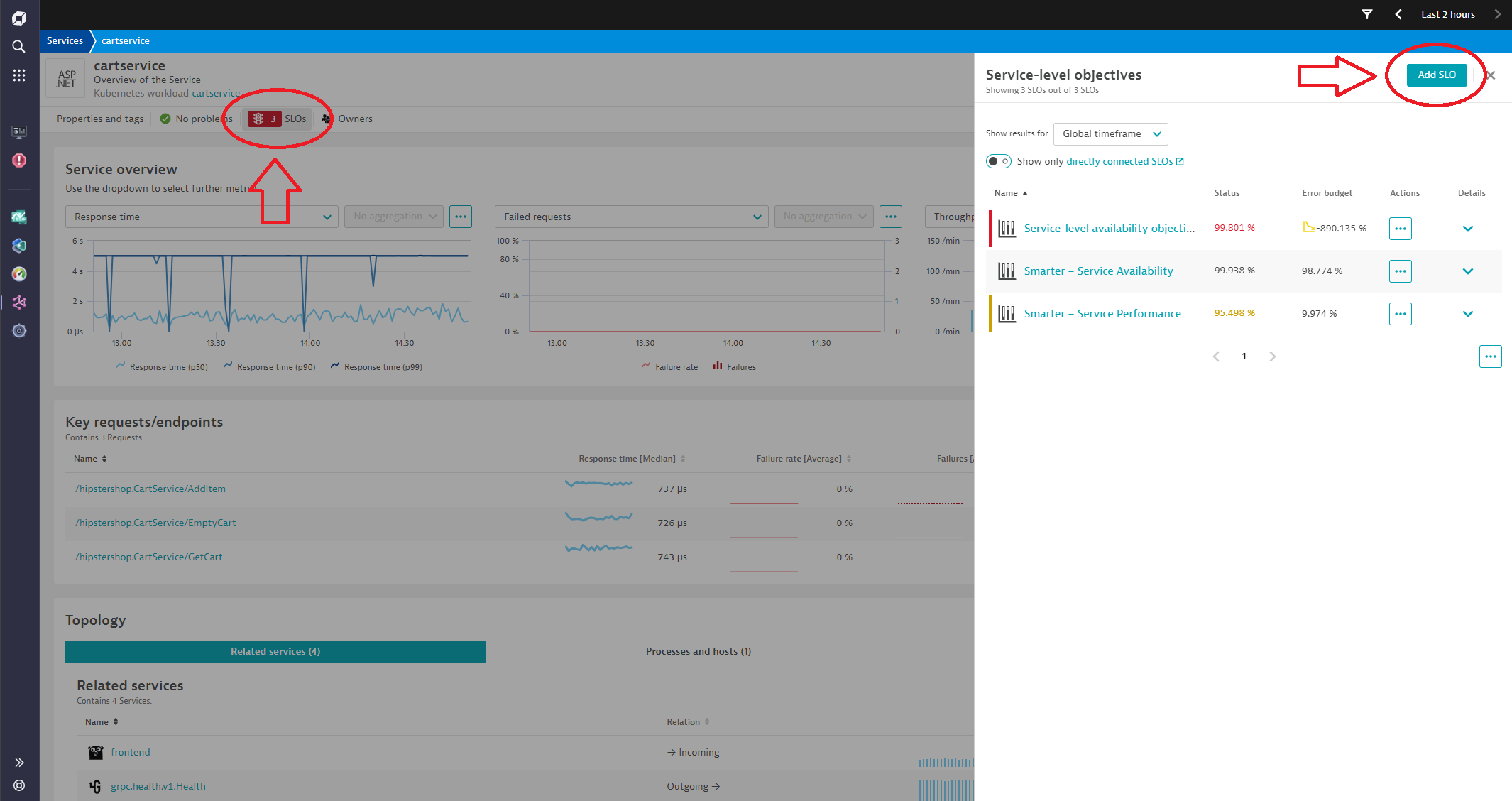

As soon as the SLO is created, it can be monitored and visualized via a dashboard. By applying alerting capabilities, a notification can be sent as soon as the service level objective is at risk of being violated.

To get more information about how SLOs can be created and support you in reaching your business goals, please have a look at the resources below:

• Service level objective examples: 5 SLO examples for faster, more reliable apps
• Lessons learned from enterprise service-level objective management
• SLOs done right: how DevOps teams can build better service-level objectives